Problem Reduction - The Most Reliable Path is Just Another Shortest Path

Applications like Google Maps or navigation systems calculate shortest paths or fastest paths all the time. There have been very efficient algorithms to solve this task since the 50s. The most reliable path can be found via the same methods – using a little trick.

Several algorithms were invented in the 50s and 60s to solve the shortest path problem. Among these were Dijkstra’s algorithm, the Bellman-Ford algorithm and a few years later the A* search algorithm. Although these algorithms are optimized for slightly varying applications, in principal, they all solve the same problem: they efficiently calculate shortest paths in a road network, or (seen from a computer scientist’s point of view) in a graph with nodes and edges.

Useful Reality Distortions

The fastest path can be calculated using a shortest path algorithm. To do this, instead of lengths (e.g. in kilometers) one simply uses the time (e.g. in hours or minutes) that will presumably be needed for each road (edge). Thus, one simply has to divide the length (s) by the expected speed (v) for each edge in the graph.

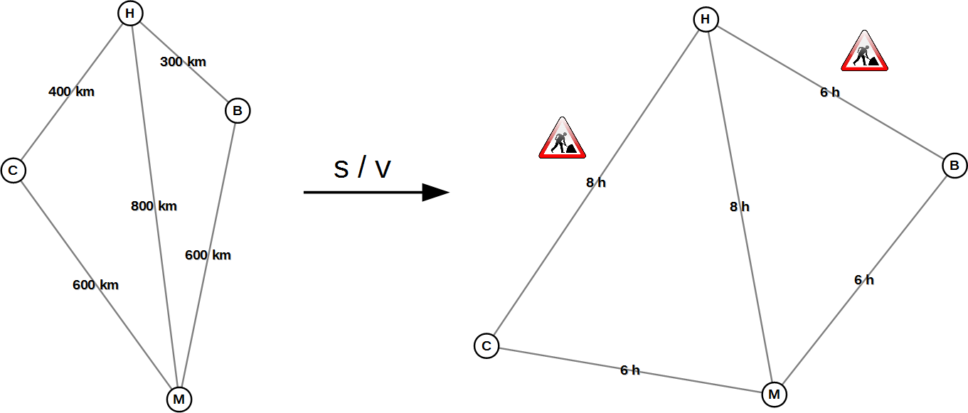
Fig. 1: The cities of Hamburg (H), Berlin (B), Cologne (C) und Munich (M). On the left a graph with the kilometers to be driven, on the right a graph with the required travel times.

Figure 1 shows an example of a transformed graph in which the time needed for each road is taken into account. We assume that you can drive 100 km/h between the cities of Hamburg, Berlin, Cologne and Munich, except on the roads Cologne-Hamburg and Hamburg-Berlin where only 50 km/h are possible due to construction works. As a result Hamburg “moves further away” from Cologne and Berlin, and the fastest way from Cologne to Berlin is now via Munich. In the transformed graph (on the right) the shortest path is also the fastest one. Thus, you can calculate the fastest way using a shortest path algorithm.

Another quite similar trick can be used to find the most reliable path. Figure 2 shows a fictitious communications network between several European countries. All edges have the probability of the communications link working properly written on them (expressed as a percentage value).

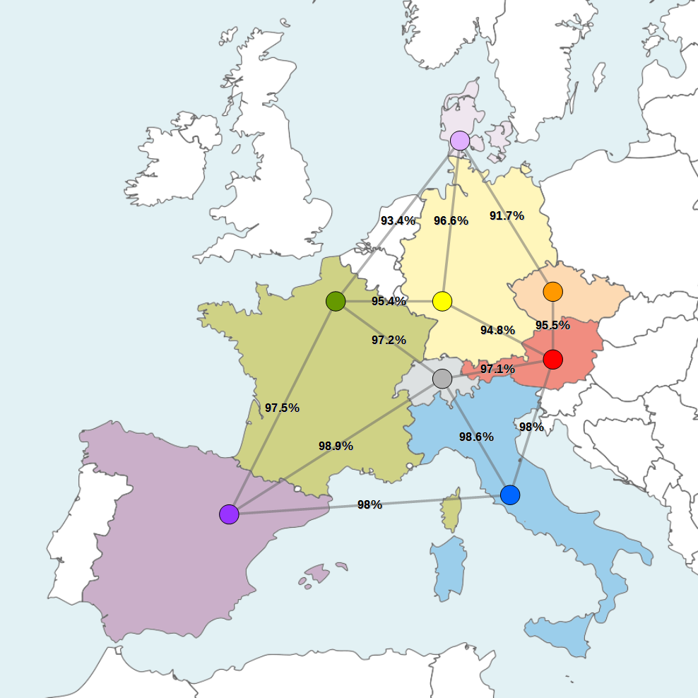
Fig. 2: Fictitious communications network between several European countries with information about reliability. The map in the background is based on Blank map of Europe by W!B, used under CC BY-SA 3.0

To calculate the reliability of a path, we have to multiply all the probabilities involved. Thus, the reliability of the path from Italy (blue) to France (green) via Switzerland (grey) is 95.8392% (=0.986 · 0.972). The most reliable path from a start node to an end node is the one where the maximum for the product of all probabilities is reached. Unfortunately, shortest path algorithms can only find paths for which the sum of all lengths of the edges is minimal. The algorithms do not quite fit our problem. Therefore, we are going to modify the problem to make it fit.

Negative Logarithm to the Rescue

For a start, let us ignore the map of Europe from figure 2 and only consider the raw data, which is the only thing we need for any calculation (see left graph in figure 3). Now we apply the negative logarithm to all percentage values. As an example, this means that between green and yellow we change the value from 0.954 (=95.4%) to -log(0.954). In figure 3 the graph on the right shows the result of this transformation. The values of the negative logarithm are visualized by the lengths of the edges. The labels (percentage values) are unchanged for clarity.

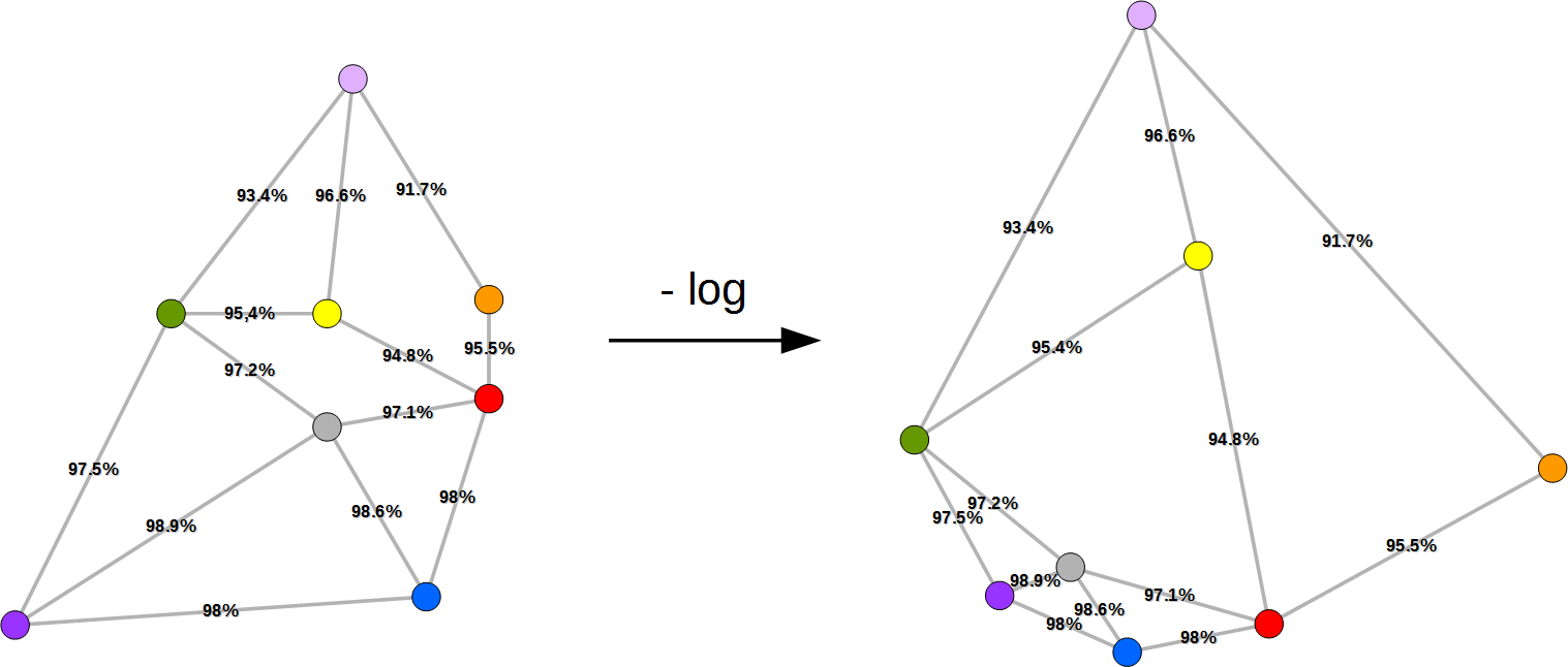
Fig. 3: Graph of the communications network before and after transforming it using the negative logarithm.

Amazingly, all shortest paths in the transformed graph (on the right) are most reliable paths. This way, one can easily recognize that the most reliable path from Austria (red) to Denmark (pale violet) is through Germany (yellow) or that the most reliable path from Austria (red) to France (green) is via Switzerland (grey). That is how the reduction of the most reliable path problem to the shortest path problem works. Pretty cool, ey?

I did not come up with this trick myself. It has been known since at least 1975 (see [1] and [2]). Although, in those days, the illustrations may not have been as nice. 🙂

Why It Works

In order to show why transforming the graph with the negative logarithm has the useful effect described above, we have to consider our problem mathematically. The following gives a mathematical formulation of the most reliable path and a step-by-step conversion of it, with each step explained:

(1) $\begin{equation*} \newcommand{\argmax}{\operatornamewithlimits{argmax}} \argmax_p \prod_{p_i \in p} p_i = ... \end{equation*}$

(1) The first term says that we are looking for the path p for which the product of its probabilities p_i has a maximum value. The function argmax expresses that we are not interested in the value of maximum reliability (in which case we would use max instead), but in the path p where said maximum reliability is reached. A subtle but important difference.

(2) $\begin{equation*} \newcommand{\argmax}{\operatornamewithlimits{argmax}} \argmax_p ( \log \prod_{p_i \in p} p_i) = ... \end{equation*}$

(2) Because the logarithm is a strictly increasing function, we can apply it without changing the solution of the maximization problem.

(3) $\begin{equation*} \newcommand{\argmax}{\operatornamewithlimits{argmax}} \argmax_p \sum_{p_i \in p} \log p_i = ... \end{equation*}$

(3) The logarithm of the product is the same as the sum of the logarithms. This is a very practical property of the logarithm. Hang in there! We are almost there!

(4) $\begin{equation*} \newcommand{\argmin}{\operatornamewithlimits{argmin}} \argmin_p ( - \sum_{p_i \in p} \log p_i) = ... \end{equation*}$

(4) Instead of looking for the maximum of the sum, we can put a minus sign before the sum and look for the minimum from now on.

(5) $\begin{equation*} \newcommand{\argmin}{\operatornamewithlimits{argmin}} \argmin_p \sum_{p_i \in p} -\log p_i \end{equation*}$

(5) Instead of negating the whole sum, we can just as well negate all the summands. What does the resulting term express? We are now looking for a path for which the sum of all edge lengths (each with -log p_i) is minimal, which again is a shortest path problem.

Conclusion

The problem of finding the most reliable path can be solved by using any shortest path algorithm. One only has to apply the negative logarithm to the probability of each edge in the graph and use the results as lengths for the shortest path algorithm.

References

CHRISTOFIDES, Nicos. Graph Theory – An Algorithmic Approach. New York: Academic Press Inc, 1975.
ROOSTA, Mohammad. Routing through a network with maximum reliability. Journal of Mathematical Analysis and Applications, 1982, 88. Jg., Nr. 2, S. 341-347.
M Roosta, J. Math. Anal. Appl., 88 (1982), pp. 341–347